Analysis

The figures are drawn by the module’s own code on a simulated sample (scripts/docs_figures.py): a doublet split by 30 µeV at 775 nm next to a single line at 776 nm, and the same doublet resolved into two lines.

① Every angle is checked

The stage reports its position only once it has settled. A position more than 0.01° from the target is commanded once more; a second miss fails the step, so no spectrum is ever recorded at the wrong angle. A step of up to 10° gets a 5 s window, a longer move 130 s, homing 180 s.

An acquisition is never repeated automatically — a repeat would expose the dot twice. The rig confirms instead that the spectrometer reported a new file.

The spectral map

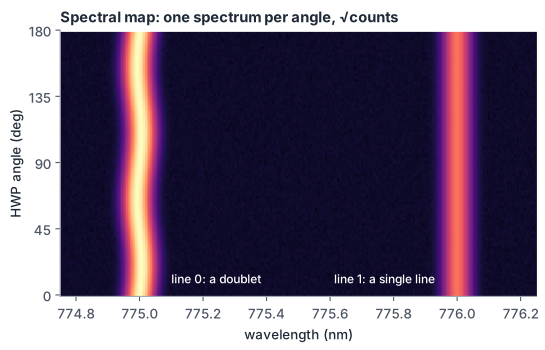
A doublet closer than its linewidth shows as one line. Its two components are polarized at right angles, so as the plate turns the polarizer passes more of one, then of the other, and the line’s centre swings between them every 90°. A single line stays where it is. The swing is a small fraction of the linewidth: it is measured by a fit, not read off the map.

② Fine structure

After the last angle of a dot, the FineStructure analyzer of plesty-fss runs in two stages: it fits every line in every spectrum, then a sine to each line’s centre against the angle.

Fitting the lines

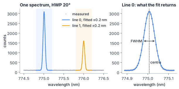
plesty-lib’s SpectrumFit, with analysis.fit_options:

1. Find the lines in the mean of all the sweep’s spectra — or, with average: median, their per-pixel median, which a cosmic ray in one spectrum does not survive. peaks names them; prominence finds every maximum standing that many counts above its surroundings.

2. Group lines closer than overlap (default 2) times the larger FWHM: those are fitted together, every other line alone. config/demo.yaml sets it high, so all its lines are fitted together.

3. Fit each group over window beyond its outer lines on each side — without one, halfway to the neighbouring groups: a Gaussian per line (model) on a linear background, by non-linear least squares. The result is each line’s centre, FWHM, height and area, each ± σ.

4. Follow the lines through the sweep: the fit to the average seeds the first spectrum, each spectrum’s fit seeds the next, in angle order; with a window the range moves with the line. center_tolerance keeps each centre that close to its seed. A spectrum whose fit fails is left out.

5. Count the signs of a fit that lost its line — failed fits, a centre or width at its bound, jumps wider than the line, outlying centres — and name every such line in warnings. Nothing is changed by the count.

analysis.fit_options	does
peaks: [775.0, 776.0]	follow the lines named, in nm
prominence: 500, average: median	follow every line found that far above its surroundings in the median spectrum
window	how much spectrum each fit sees beyond its lines, in nm
center_tolerance	how far a centre may move from one spectrum to the next, in nm
width_bounds	the FWHM range a line may take, in nm
overlap, model	when lines are fitted together; the line shape — gaussian, lorentzian or voigt

Fitting the fine-structure curve

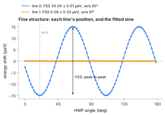
Each line’s centres are fitted with

centre(θ) = mean + A · cos(k · (θ − axis))

where k comes from analysis.rotator: 4 for a half-wave plate (a 90° period), 2 for a rotating polarizer (180°). Written as mean + a·sin(kθ) + b·cos(kθ), the model is linear in mean, a and b, so the fit is a weighted linear least-squares solve — no starting values, nothing to fail to converge. Each centre is weighted by 1/σ² of its line fit, and the errors are scaled by the reduced χ².

• FSS = 2A, the peak-to-peak, turned into an energy at the mean position: ΔE = hc · 2A / mean², in µeV, its error from the fit’s full covariance.

• axis = atan2(a, b) / k: the plate angle where the line sits at its longest wavelength — its lowest energy.

• fss_valid = 2A is smaller than the line’s median FWHM. A swing as wide as the line means the fit followed different lines, not one doublet.

• Fewer than four fitted spectra leave everything nan.

What it reports

Output	Holds
the dot’s analysis record in records.jsonl	per line center, fss_ueV, fss_err_ueV, fss_valid, axis_deg; warnings
analysis/<dot>_line_fit	every line’s fit in every spectrum: centre, width, height, their errors
analysis/<dot>_fine_structure	per line the FSS, axis and mean centre with errors, the fit’s R², fss_valid
analysis/<dot>.report.json	a sentence, a table of the lines and the sweep drawn

The saved outputs load with ExperimentData.load. The report renders with plesty.lib.report.Report.load(path).to_html(), without importing plesty-fss.

How to read them

A good result — the figures above. The map shows the doublet as one line with a gentle 90° wiggle. In the fine-structure plot the points lie on the sine; the FSS is many times its error, and warnings is empty. A single line gives an FSS indistinguishable from 0.

A doublet resolved into two lines — no splitting to trust:

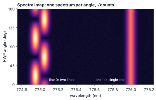
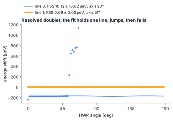
The map shows two lines handing the intensity back and forth instead of one line swinging. The fit of line 0 holds one of them, jumps when its intensity fades, then stops converging; the FSS comes out smaller than its error and the analysis names the line in warnings. A line whose centre swings by at least its linewidth is marked fss_valid: false. Either way, the splitting is the distance between the two lines, read off the spectrum — not this fit.

You see	It means
points on a clean sine, error ≪ FSS	a splitting measured
flat points, FSS ≈ 0 within its error	an unsplit line, or the axis along the polarizer
scattered points, error ≥ FSS, a warning	the fit lost the line: resolved doublet, a neighbour, or too weak — check prominence
fss_valid: false	the swing is as wide as the line: not one line any more